Top 10 Excel Formatting Tips To Make Your Life Easier

Do you know how sometimes looking at a bunch of numbers and letters on a computer screen can be confusing and messy? It’s like trying to understand ancient writing, and that’s strange. But don’t worry! There’s a secret trick that can help. It’s called formatting.

Formatting is like putting makeup on your data. It doesn’t change what the numbers and letters mean, but it makes them look much nicer and easier to understand.

With a few simple excel formatting tips and tricks, you can turn your messy lists into neat and professional-looking documents that anyone can understand.

And here’s the cool part: formatting isn’t just about making things look good (although that’s a nice bonus!). It also helps you work faster and smarter. 

Highlighting the important stuff makes it easy to find what you need quickly. Plus, well-formatted lists are easier to share and work on with other people.

So, if you’re tired of struggling with messy data, let’s learn how to make it look great together!

Why Do We Even Need To Format Our Excel Sheet?

Think of your spreadsheet as a room full of boxes. Without organizing, it’s a mess. Formatting is like tidying up those boxes, labeling them clearly, and even coloring them. 

Here’s why formatting is your spreadsheet’s superhero:

• See Clearly: Formatting makes your data look neat and organized. Using bold headings, aligning numbers neatly, and adding borders make it simple to look at your document and find what you need quickly. No more searching around!

• Understand Numbers: Have you ever tried to figure out if a number is a price, percentage, or date? Well, using decimals, percent signs, and date formats makes it crystal clear what each number represents. No more confusion!

• Highlight the Important Stuff: Conditional formatting helps you highlight important data by using colors. For example, imagine your sales numbers are shown in either green or red. With this formatting, you can quickly see which products are performing well and which ones are not, making it simple to notice any patterns or trends.

• Save Time and Stress: Formatting makes your work easier. Imagine a magic tool that lets you quickly apply styles to many cells together instead of doing it one by one. That means less time spent on each cell!

• Impress Everyone: A nicely organized spreadsheet looks really good and shows you’re careful and professional. It makes your work stand out and could even lead to praise or a promotion!

Next time you’re in Excel, don’t shy away from formatting tools. You’ll be surprised how much easier and enjoyable it is to work with your data. 

Top 10 Excel Formatting Tips To Make Your Life Easier

Let’s get started with our top 10 Excel formatting tips:

1. How To Change Color Quickly

Want to switch up the colors in your spreadsheet or dashboard? Here’s how: Go to the Page Layout tab and click on the Colors box in the top left corner. 

Microsoft offers preset color schemes that look good and stand out on your screen. You can also make your color schemes to match your company’s style. 

Plus, you can customize font colors too or mix and match colors and fonts to create your unique theme.

2. How to Use Bold and Italic

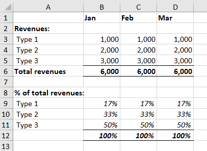
To make certain parts of your data stand out more in a spreadsheet, you can use bold text for emphasis and italic text for special information, like percentages. For example, on a monthly cash flow sheet, you might want to make the totals bold and show percentages in italics, like this:

Here’s how you can do it:

• Select the cells you want to make bold or italic.
• Go to the Home tab and find the Bold and Italic icons in the Font section.
• Click the icon you need. You can even click both icons if you want to format the text in both directions.

3. Easily reset your spreadsheet

Do you ever need to fix a messy spreadsheet? Maybe your coworker messed up the budget file. What do you do?

It’s easy. Select all the cells, then go to Home > Clear > Clear Formats. This will remove all the styling, so you can start fresh and format it however you like.

4. Formatting Options For Print

Use the right print settings to ensure that your printed documents look as good as they do on your screen. These settings are in the Page Layout ribbon. 

To see how your document will look before printing, use the print preview feature and click on the “page settings” button for more options.

5. How to Use Text Colors

Here’s an easier way to understand how to use different colors for text in Excel:

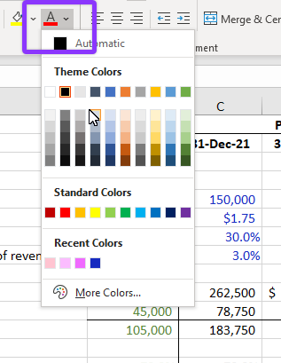
When you color code text in Excel, it helps you quickly understand what the numbers mean. Here’s what each color usually represents:

• Blue is for constant numbers, like old data or guesses.
• Black is for formulas that use numbers from the same Excel sheet.
• Green is for formulas that get numbers from a different sheet in the same file.
• Red is for formulas that use numbers from a different file.

To color your text:

• Click on the cell or cells you want to color.
• Go to the Home tab at the top.
• Look for the icon that lets you change the text color.
• Choose the color you want from the options provided.

Read More: Top 30 Excel Tips & Tricks to Make You an Excel Pro!

6. How to Format Data as a Table

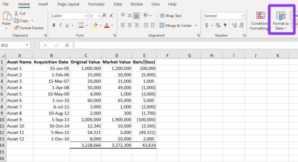
Excel’s table feature helps organize large sets of data so they’re easier to understand and work with. Let’s say you have a bunch of information about assets like when they were acquired, their original value, and their current market value. You can turn this data into a table by following these steps:

1. First, select any cell within the range of your data.

2. Then, go to the Home tab and click on the icon that says “Format as Table.”

3. You’ll see a bunch of different styles to choose from. Pick one that you like.

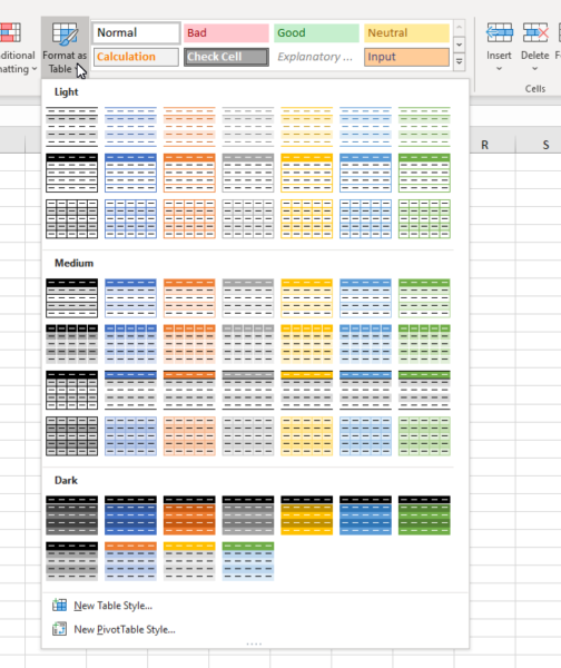
4. If your data contains no empty cells, Excel will automatically determine the range. Otherwise, you’ll have to tell it which cells to include.

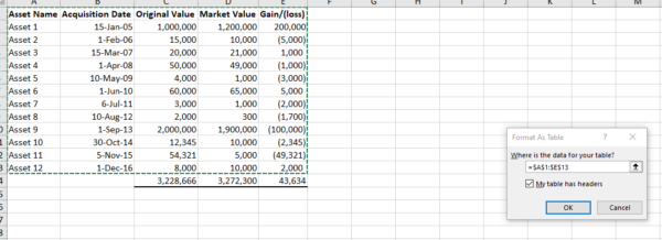
5. Make sure you check the box that says “My Table Has Headers.”

6. Click OK, and Excel will create the table for you.

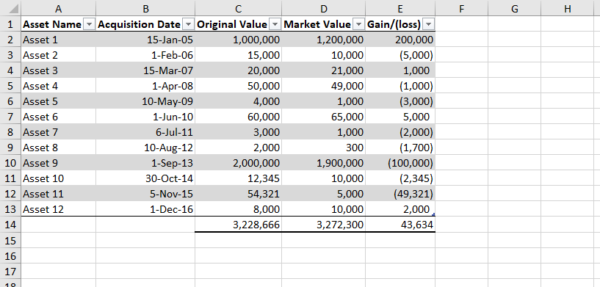
Now, your data is much easier to read and work with. You can sort or filter the information in any column by clicking on the little drop-down arrow in the header. And there are even more features and options you can try out to make working with your data even smoother.

7. How to Format Percentages

In spreadsheets, percentages are often used to show parts of a whole. For instance, if you’re looking at different sources of income, you might want to see what percentage each source contributes to the total revenue.

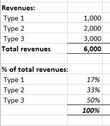
To show percentages in your spreadsheet:

1. Select the cells you want to work with.
2. Go to the “Home” tab.
3. Look for the “Number” section.
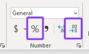
4. Click on the “Percent Style” icon.
5. This will automatically add two decimal places to your numbers. If you don’t want decimals, click the “Decrease Decimals” icon twice.

8. How to Format Dates

It’s really important to put dates in your financial documents like spreadsheets. Dates help you understand when things happened, like when money came in or went out.

Different people like to see dates in different ways. Some prefer to see the full date written out, like “December 31, 2019.”

If you’re using Excel, it’s easy to change how dates look. Here’s how:

1. Go to the “Home” tab in Excel.

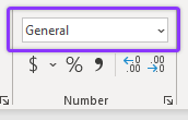
2. Look for the box where it says “Number Format” and click on it. A menu will pop up.

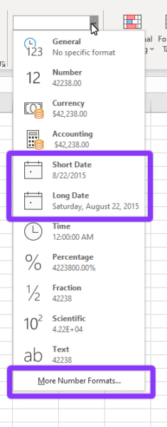
3. You’ll see two options for dates: “Short Date” and “Long Date.”

4. If you want even more choices, click on “More Number Formats.”

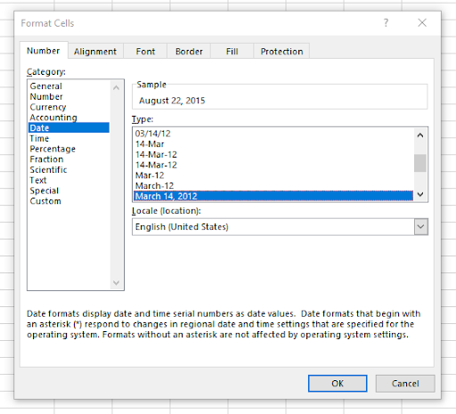
5. In the new box that appears, choose “Date” on the left side. Then, select the date style you like.

6. Click “OK” when you’re done.

9. How to Copy Formatting With the Fill Handle

The Fill Handle is a little square at the bottom right corner of a cell you’ve picked. When you put your mouse over it, it changes into a black cross.

You can use the Fill Handle to copy a cell’s appearance and use that style in other cells next to it. However, copying across rows is different from copying down columns.

Let’s say you’re making a table for your monthly money stuff. The months are at the top, and the things you’re getting and spending money on are on the side. You put a number in the first box and want all the other boxes to look the same.

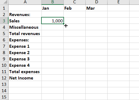
To copy the format in a row, follow these steps:

1. Click on the cell with the format you want to copy.
2. Move your mouse over the Fill Handle (a small square at the bottom right corner of the cell).
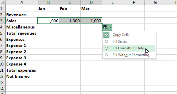
3. Drag the Fill Handle across the row until you reach the last cell you want to format.
4. When you release the mouse, a black cross will appear, indicating the copy action.
5. But wait! You only want to copy the format, not the numbers.
6. Click on the Auto Fill Options icon that appears next to the last copied cell.
7. Choose “Fill Formatting Only” from the menu that pops up.
8. Now, the numbers will disappear from the cells you copied, leaving only the original format.

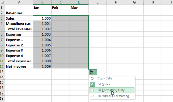
First, do what you did in the first row to the other rows:

1. Put your cursor on the first row and make it stand out.
2. Hover your mouse over the Fill Handle and double-click it.
3. The cells below will fill up with the same style as the first row.
4. Click on the Auto Fill Options icon and pick Fill Formatting Only. This will remove the numbers, leaving only empty, formatted cells.

10 Formatting Tricks Only Excel Experts Would Know

Here are 10 extra ways to make your Excel sheets look fantastic! 

• Center Across Selection: Merge cells without actually merging them.
• Merge Across: Combine multiple cells horizontally.
• Custom Cell Formatting: Hide decimal points for large numbers or display numbers in thousands or millions.
• New Line in a Cell: Use ALT+Enter to create a new line within a cell.
• Paste Special: Copy only the widths of cells for precise formatting.
• Custom Chart Labels: Skip displaying zero values in chart labels.
• Alignment Tools: Align and distribute charts with ease.
• Custom Time Format: Display total hours using the [h]: mm custom code.
• Text Format for Long Numbers: Format very long numbers as text to avoid truncation.

Shortcut Keys to Format Data in Excel

Here are some easy shortcuts for formatting data in Excel:

• Bold Text: Press Ctrl and 2 or Ctrl and B together to make your text bold.
• Italic Text: Press Ctrl and 3 or Ctrl and I together to make your text italic.
• Underline Text: Press Ctrl and 4 or Ctrl and U together to underline your text.
• Alignment Options: Press Alt and H, then A, to center-align your text.
• Font Size: Press Alt and H, then G, to make your text bigger, or Alt and H, then K, to make it smaller.
• Border: Press Alt and H, then B, to add a border around your cells.
• Format Cells: Press Ctrl and 1 to open a menu where you can change many formatting options.
• Outline Border: Press Ctrl, Shift, and the Ampersand (&) keys together to outline selected cells.
• Percentage Format: Press Ctrl, Shift, and the Percent (%) keys together to apply a percentage format.
• Strikethrough: Press Ctrl and 5 to add or remove strikethrough from your text.

Wrap Up

In short, knowing how to format in Excel is really important for people who use spreadsheets. It makes your work look better and helps you understand and analyze data better, too. 

By using these tips, you can make Excel work even better for you. Your spreadsheets will be clearer, more professional, and better for making decisions and sharing information. 

So, when you use Excel next time, don’t forget how formatting can make your data easier to understand. Have fun formatting!

FAQs