Ever felt lost while scrolling through a huge Excel spreadsheet? Say goodbye to those frustrating moments! This guide will show you how to freeze rows, a trick that will make your Excel experience much easier.
Imagine you’re looking at a big dataset with lots of rows and columns. But as you scroll, the important header row with all the labels keeps disappearing. Annoying, right? Freezing rows can help! This simple trick locks certain rows in place so they stay visible no matter how far you scroll.
Interested? Keep reading to learn how to freeze rows in Excel and master your spreadsheets!
What does it mean to freeze a row in Excel?
Freezing a row in Excel means locking that row so it stays visible when you scroll through the spreadsheet. This feature helps keep important information, like headers, in view no matter where you navigate on the sheet.
Freeze panes allow you to lock both rows and columns in place. This means that these rows and columns remain visible as you scroll down or across your sheet. It’s a useful tool because Excel sheets can have up to 1,048,576 rows and over 16,000 columns, making it easy to lose track of your data.
Here’s why freezing rows is useful:
- Maintains Context: In large datasets, scrolling can make it hard to remember which data belongs to which column. Freezing the header row keeps the labels visible, so you always know what each column represents.
- Improves Readability: In spreadsheets with many columns, frozen rows keep the headers in view, making it easier to identify the data in each column.
- Easier Comparison: When dealing with extensive data, freezing a row with important information like averages or totals lets you compare it with values in other rows throughout the spreadsheet.
Overall, freezing rows in Excel makes working with large datasets more user-friendly and efficient.
How to Freeze Rows in Excel – Simple & Easy Way
Freezing rows in Excel is easy. Here’s how you can do it:
Freeze the Top Row
To lock the first row (row 1):
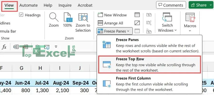
- Go to the View tab.
- Click on Freeze Panes.
- Select Freeze Top Row.

This keeps the first row visible as you scroll down.
Freeze Multiple Rows
To freeze rows 1 and 2:
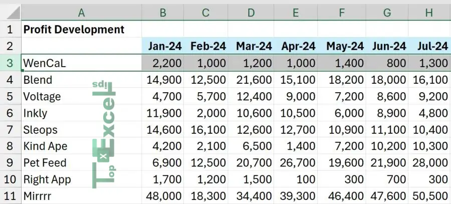
1. Select row 3 (the row right below the ones you want to freeze).

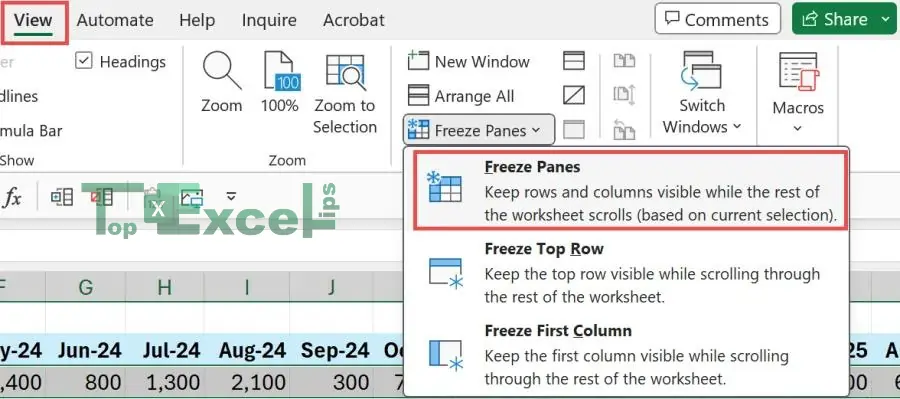
2. Go to the View tab.
3. Click on Freeze Panes.

4. Choose Freeze Panes from the drop-down menu.
Now, rows 1 and 2 will stay visible as you scroll down the worksheet. For example, if you scroll down to row 35, rows 1 and 2 will still be in view.
Must Read: How To Separate Names In Excel (3 Easy Ways)
How to Freeze a Row in Excel That Is Not the Top Row
If you want to freeze a row in Excel that is not the top row, follow these steps:
- Select the Row Below the One You Want to Freeze
- Click on the row number directly below the row you want to freeze. For example, if you want to freeze row 5, select row 6.
- Go to the View Tab
- Navigate to the View tab on the ribbon at the top of Excel.
- Freeze Panes
- Click on Freeze Panes.
- From the drop-down menu, choose Freeze Panes.
This will lock all rows above the selected row, keeping them visible as you scroll. For instance, if you selected row 6, rows 1 through 5 will remain visible as you move through the worksheet.
How to Freeze a Row in Excel With Shortcut Method
To freeze a row in Excel using a shortcut:
- Select the Row Below the One You Want to Freeze
- Click on the row number directly below the row you want to freeze. For example, if you want to freeze row 5, select row 6.
- Use the Shortcut
- Press Alt + W + F + R sequentially on your keyboard.
This shortcut will freeze all rows above the selected row, keeping them visible as you scroll.
How to Unfreeze Panes in Excel
Returning your worksheet to its original layout by unfreezing panes is straightforward. Here’s how:
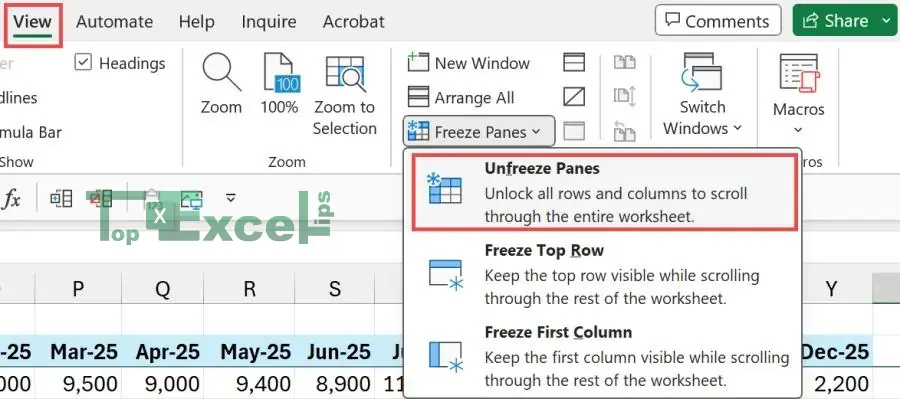
- Go to the View Tab
- Navigate to the View tab located on the ribbon at the top of Excel.
- Access Freeze Panes
- Click on Freeze Panes.
- Select Unfreeze Panes
- From the drop-down menu, choose Unfreeze Panes.

This action will remove the frozen panes, allowing your worksheet to return to its default view.
Must Read: Top 101+ Excel Shortcuts Cheat Sheet That You Love + PDF
Wrap Up
Freezing rows in Excel is a valuable feature that boosts productivity and efficiency when handling large datasets.
By keeping important information, like headers or labels, always visible, you can maintain context, enhance readability, and make it easier to compare different rows and columns.
This guide offers step-by-step instructions, including a shortcut method, to help you freeze the top row, multiple rows, or even rows that are not at the top of the worksheet.
With frozen rows, you can navigate through your spreadsheets confidently, ensuring that crucial information stays accessible and visible. This ultimately streamlines your workflow, enabling more effective data analysis and manipulation.
FAQs
How to Freeze a Row and a Column at the Same Time
To freeze both rows and columns:
1. Click the cell that is below the rows and to the right of the columns you want to freeze.For example, to freeze rows 1 to 3 and columns A to C, select cell D4.
2. Go to the View tab.
3. Click on the Freeze Panes drop-down.
4. Select Freeze Panes.
These steps will keep your selected rows and columns visible while you scroll through the rest of your worksheet.
How do I freeze random rows in Excel?
To freeze random rows in Excel, first, select or highlight the row directly below the set of rows you wish to freeze. Then, navigate to the menu at the top of the spreadsheet and click on the ‘View’ tab. Once the sub-menu appears, locate and click on the ‘Freeze Panes’ button. This action will effectively freeze the rows above the selected row, allowing you to scroll through your spreadsheet while keeping those rows visible.


