Excel is a powerful tool for managing data, but sometimes you need to hide or unhide rows to keep your information organized.
This guide explains what unhiding rows means in Excel and why it’s essential to know how to do it.
We’ll cover various methods to unhide rows, including shortcuts and step-by-step instructions, as well as how to fix common issues when unhiding doesn’t work.
What Is Unhide in Excel?
In Excel, the “unhide” function makes hidden cells, columns, and rows visible again. This function undoes the “hide” action, which conceals parts of the worksheet without deleting them.
People use the hide function to protect sensitive data or to focus on specific parts of the worksheet. You can hide entire columns or rows, but not individual cells.
Why Learning Excel Is Important
Knowing how to use Excel is crucial in today’s business world. It’s an excellent tool for sorting and analyzing large amounts of data.
However, when working with hundreds or thousands of rows and columns, the worksheet can become overwhelming. Hiding certain parts can simplify the view and make the data easier to work with.
The Benefits of Unhiding Rows in Excel
For beginners, learning to unhide rows is very useful for organizing data and managing spreadsheets.
- Control Visibility: Unhiding rows lets you control what you see in your worksheet, making it easier to find and analyze information.
- Quick Access: It allows you to quickly view all the information in hidden rows, saving time compared to unhiding each row individually.
By mastering the unhide function, you can manage your Excel worksheets more effectively and efficiently.
Must Read: Top 101+ Excel Shortcuts Cheat Sheet That You Love + PDF
How to Unhide All Rows in Excel
Unhiding rows in Excel is straightforward:
- Go to the Home tab.

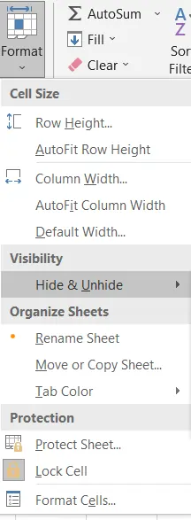
2. Click on “Format” in the Menu.
3. Go to “Visibility” and select “Hide & Unhide.”
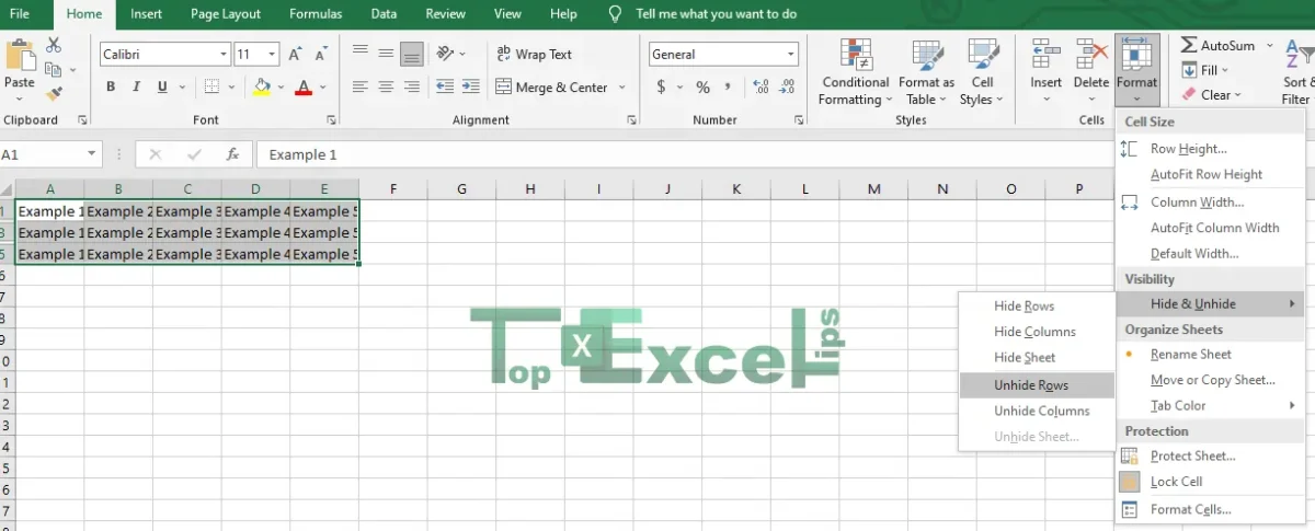
4. Click on “Unhide Rows.”
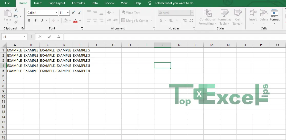
Alternatively, you can use the keyboard shortcut “Ctrl + Shift + (” to unhide rows.)
How to Unhide Specific Rows in Excel
To unhide specific rows:
- Select the rows above and below the hidden rows.
- Right-click and choose “Unhide” from the menu.
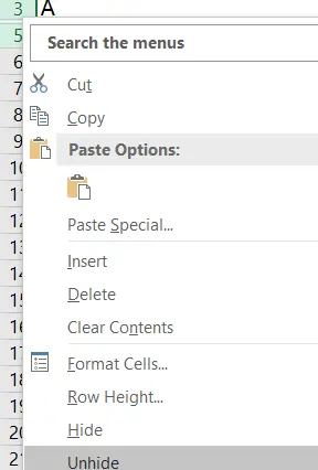
That’s it! The hidden rows will become visible using these methods.
How to Unhide Multiple Rows in Excel
Step 1: Select Visible Cells
- Go to the Home tab.
- Select all the visible cells that include the hidden rows.
Step 2: Access Format Menu
- Click on the Format menu.
Step 3: Navigate to Hide & Unhide
- Under the Format menu, find the Visibility option.
- Choose ‘Hide & Unhide‘ from the sub-options.
Step 4: Unhide Rows
- Click ‘Unhide Rows‘ in the dropdown menu.
Shortcut Method
- You can also press “Ctrl + Shift + (” to unhide rows quickly.)
Step 5: Confirm Unhiding
- Once you click ‘Unhide Rows‘, the hidden rows will become visible again.
Must Read: How To Separate Names In Excel (3 Easy Ways)
How to Unhide All Rows in Excel With a Shortcut
To reveal all hidden rows in Excel using a shortcut:
1. Open your Excel spreadsheet.
2. Navigate to the worksheet where rows are hidden.
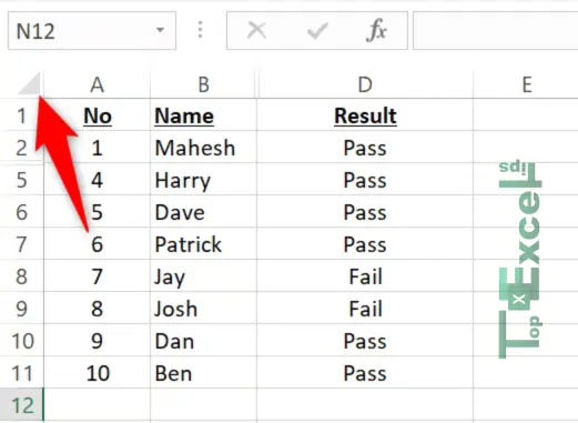
3. Select the entire worksheet by pressing Ctrl+A (Windows) or Command+A (Mac). Alternatively, you can click the “Select All” button located in the top-left corner of the worksheet.
4. With the worksheet selected, use the shortcut Ctrl+Shift+9. This command will unhide all hidden rows instantly.
5. Alternatively, you can right-click on any selected cell within the worksheet and choose “Unhide” from the context menu to achieve the same result.
Following these steps will allow you to quickly unhide all rows in Excel using either a keyboard shortcut or the right-click menu.
How to Fix Unhide Rows in Excel Not Working
Here are steps to fix issues with unhide rows in Excel when it’s not working:
If the Freeze Panes Option is Active:
- Navigate to the View tab.
- Click on “Freeze Panes” in the dropdown list and select “Unfreeze Panes.”
- Alternatively, use the keyboard shortcut ALT + W + F + F.
- Your rows should now be visible, and hiding/unhiding should work properly from now on.
When the Row Height is Very Small or Zero:
- Right-click on the row number where rows are hidden.
- Choose “Row Height” from the menu.
- Increase the row height as needed to reveal the hidden rows.
If Filter Mode is Active:
- Go to the Data tab.
- Under the Sort & Filter ribbon, select “Clear” in the “Filter” group.
- This action will remove any hidden rows caused by active filters, making all rows visible again.
Must Read: How To Freeze A Row In Excel That Is Not the Top Row
Wrap Up
Knowing how to unhide rows in Excel is a valuable skill for anyone working with spreadsheets.
Whether you need to unhide all rows at once, reveal specific rows, or troubleshoot when the unhide function isn’t working, these techniques will help you manage your data more effectively.
With practice, you’ll be able to control the visibility of your data and work more efficiently in Excel.
FAQs
How do I check for frozen panes in Excel?
To keep part of your worksheet visible while scrolling, follow these steps:
1. Go to the View tab.
2. Select Freeze Panes to lock specific rows and columns in place.
3. Alternatively, choose Split Panes to create two separate windows of the same worksheet.
How to unhide all rows in Excel on a Mac?
Unhiding rows on a Mac is the same as on Windows:
1. Select the hidden rows by dragging your cursor over them.
2. Right-click and select Unhide.
What does it mean if the Unhide option is gray?
If the Unhide option in your Format list is gray, it means it’s not available. Here are two possible reasons:
1. Protected Worksheet: You might be working on a protected worksheet. To unprotect it, go to the Review tab, click on Changes, and select Unprotect Sheet. This should make the Unhide button clickable.
2. No Hidden Items: If the worksheet is already unprotected, a gray Unhide button might mean there are no hidden items to unhide.
Do I need to adjust the height of rows after unhiding?
No, you don’t need to adjust the row height after unhiding, as long as the row height properties haven’t been changed.


